机器学习基础术语
学习机器学习就像学习一门新语言,需要先掌握基本词汇。这些术语构成了机器学习的"语言系统",理解它们是深入学习的第一步。
想象一下你在教一个机器人认识水果:
- 数据:各种水果的图片和信息
- 特征:水果的颜色、形状、大小、味道
- 标签:这个水果叫什么名字(苹果、香蕉、橙子)
- 模型:机器人学到的"识别水果的方法"
- 训练:教机器人认识水果的过程
- 推理:机器人识别新水果的能力
数据(Data)
什么是数据?
数据是机器学习的"原材料",就像厨师做菜需要的食材一样。没有数据,机器学习就无法进行。

数据的类型
1. 结构化数据
特点:有明确的格式和组织方式,像表格一样整齐
# 结构化数据示例:学生信息表实例
import pandas as pd
students_data = {
'姓名': ['张三', '李四', '王五'],
'年龄': [18, 19, 20],
'成绩': [85, 92, 78],
'班级': ['一班', '二班', '一班']
}
df = pd.DataFrame(students_data)
print(df)
students_data = {
'姓名': ['张三', '李四', '王五'],
'年龄': [18, 19, 20],
'成绩': [85, 92, 78],
'班级': ['一班', '二班', '一班']
}
df = pd.DataFrame(students_data)
print(df)
输出:
   姓名  年龄  成绩  班级
0  张三  18  85  一班
1  李四  19  92  二班
2  王五  20  78  一班
2. 非结构化数据
特点:没有固定格式,需要特殊处理
例子:
- 文本:评论、文章、邮件
- 图像:照片、医学影像
- 音频:语音、音乐
- 视频:监控录像、电影
# 非结构化数据示例:文本和图像
text_data = "这个产品质量很好,我很满意!"
# image_data = 一张产品的照片
# audio_data = 顾客的语音评价
数据质量的重要性
垃圾进,垃圾出(Garbage In, Garbage Out)是机器学习的重要原则。数据质量直接决定模型效果。
实例
# 数据质量问题示例
import numpy as np
import pandas as pd
# 创建包含各种问题的数据
problematic_data = {
'价格': [100, 200, None, 300, -50], # 缺失值和异常值
'评分': [4.5, '好', 3.8, 4.2, 5.0], # 数据类型不一致
'销量': [1000, 1200, 800, 1500, '很多'] # 文本和数字混合
}
df = pd.DataFrame(problematic_data)
print("有问题的数据:")
print(df)
print("\n数据问题分析:")
print(f"缺失值数量:{df.isnull().sum().sum()}")
print(f"数据类型:\n{df.dtypes}")
特征(Feature)
什么是特征?
特征是数据的"可观察属性",就像描述一个人的特征:身高、体重、发色、性格等。在机器学习中,特征是用来做预测的依据。
特征选择的重要性:
- 好的特征能让模型事半功倍
- 坏的特征会让模型事倍功半
- 特征工程往往是决定模型效果的关键
特征的类型
x1. 数值特征
特点:可以用数字表示,可以进行数学运算
# 数值特征示例
numerical_features = {
    '年龄': [25, 30, 35, 40],
    '收入': [5000, 8000, 12000, 15000],
    '身高': [165, 170, 175, 180]
}
2. 类别特征
特点:表示不同的类别,不能进行数学运算
# 类别特征示例
categorical_features = {
    '性别': ['男', '女', '男', '女'],
    '学历': ['本科', '硕士', '博士', '本科'],
    '城市': ['北京', '上海', '广州', '深圳']
}
3. 文本特征
特点:需要特殊处理才能被模型使用
# 文本特征示例
text_features = {
    '评论': [
        '这个产品很好用,推荐购买!',
        '质量一般,不太满意。',
        '性价比高,值得入手。'
    ]
}
特征工程示例
实例
# 特征工程示例:从原始数据创建有用特征
import pandas as pd
import numpy as np
# 原始数据:房屋信息
house_data = {
'面积': [80, 120, 60, 150, 90],
'卧室数': [2, 3, 1, 4, 2],
'建造年份': [2000, 2010, 1995, 2015, 2005],
'价格': [200, 350, 150, 500, 280]
}
df = pd.DataFrame(house_data)
# 创建新特征
df['房龄'] = 2023 - df['建造年份'] # 房屋年龄
df['每平米价格'] = df['价格'] / df['面积'] # 单价
df['卧室面积比'] = df['卧室数'] / df['面积'] * 100 # 卧室占比
print("原始数据 + 新特征:")
print(df)
# 特征重要性分析
correlation = df.corr()['价格'].sort_values(ascending=False)
print("\n特征与价格的相关性:")
print(correlation)
标签(Label)
什么是标签?
标签是我们想要预测的"答案",就像考试题的正确答案一样。在监督学习中,每个数据样本都有一个对应的标签。
标签的作用:
- 指导模型学习方向
- 评估模型学习效果
- 定义问题的类型
标签的类型
1. 分类标签
特点:离散的类别值
# 分类标签示例
classification_labels = {
    '邮件类型': ['垃圾邮件', '正常邮件', '垃圾邮件', '正常邮件'],
    '情感倾向': ['正面', '负面', '中性', '正面'],
    '疾病诊断': ['患病', '健康', '健康', '患病']
}
2. 回归标签
特点:连续的数值
# 回归标签示例
regression_labels = {
    '房价': [250000, 320000, 180000, 450000],
    '温度': [25.5, 28.3, 22.1, 30.0],
    '股票价格': [100.5, 105.2, 98.7, 110.3]
}
标签质量的重要性
# 标签质量问题示例
import numpy as np
# 模拟图像分类任务中的标签问题
image_data = ['cat1.jpg', 'dog1.jpg', 'cat2.jpg', 'dog2.jpg']
problematic_labels = ['猫', '犬', '猫咪', '狗']  # 标签不一致
# 标签标准化
label_mapping = {
    '猫': 'cat', '猫咪': 'cat',
    '犬': 'dog', '狗': 'dog'
}
standardized_labels = [label_mapping[label] for label in problematic_labels]
print("原始标签:", problematic_labels)
print("标准化标签:", standardized_labels)
模型(Model)
什么是模型?
模型是机器学习算法从数据中学到的"规律"或"模式",就像学生从课本中学到的知识一样。
模型的本质:
- 数学函数:输入特征,输出预测
- 参数集合:学到的规律的具体表示
- 决策规则:如何从输入得到输出
模型的表示
实例
# 简单线性模型示例
import numpy as np
import matplotlib.pyplot as plt
# 模拟数据
X = np.array([1, 2, 3, 4, 5])
y = np.array([2, 4, 6, 8, 10])
# 线性模型:y = w * x + b
# 学习到的参数:w = 2, b = 0
w, b = 2, 0
def linear_model(x):
"""线性模型函数"""
return w * x + b
# 预测
predictions = linear_model(X)
# 可视化
plt.scatter(X, y, color='blue', label='真实数据')
plt.plot(X, predictions, color='red', label='模型预测')
plt.xlabel('输入 X')
plt.ylabel('输出 y')
plt.title('线性模型示例')
plt.legend()
plt.grid(True)
plt.show()
print(f"模型参数:w = {w}, b = {b}")
print(f"预测结果:{predictions}")
模型的复杂度
实例
# 模型复杂度对比
from sklearn.preprocessing import PolynomialFeatures
from sklearn.linear_model import LinearRegression
import numpy as np
# 生成非线性数据
np.random.seed(42)
X = np.random.rand(20, 1) * 10
y = np.sin(X) + np.random.randn(20, 1) * 0.1
# 简单模型(线性)
simple_model = LinearRegression()
simple_model.fit(X, y)
# 复杂模型(高次多项式)
poly_features = PolynomialFeatures(degree=10)
X_poly = poly_features.fit_transform(X)
complex_model = LinearRegression()
complex_model.fit(X_poly, y)
# 可视化
X_test = np.linspace(0, 10, 100).reshape(-1, 1)
X_test_poly = poly_features.transform(X_test)
plt.scatter(X, y, color='blue', label='训练数据')
plt.plot(X_test, simple_model.predict(X_test), color='green', label='简单模型')
plt.plot(X_test, complex_model.predict(X_test_poly), color='red', label='复杂模型')
plt.xlabel('X')
plt.ylabel('y')
plt.title('模型复杂度对比')
plt.legend()
plt.grid(True)
plt.show()
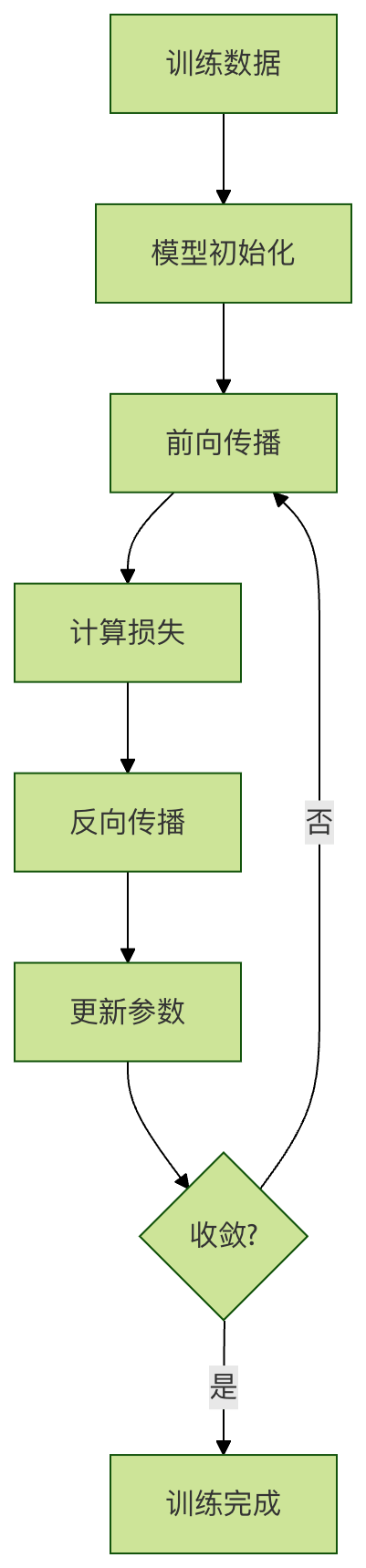
训练(Training)
什么是训练?
训练是模型学习的过程,就像学生上课学习知识一样。在训练过程中,模型不断调整参数,使预测结果越来越接近真实标签。
训练过程示例
实例
# 训练过程示例:简单线性回归
import numpy as np
import matplotlib.pyplot as plt
# 生成训练数据
np.random.seed(42)
X = np.random.rand(50, 1) * 10
y = 3 * X + 2 + np.random.randn(50, 1) * 2
# 初始化模型参数
w, b = 0.0, 0.0
learning_rate = 0.01
epochs = 100
# 记录训练过程
loss_history = []
# 训练循环
for epoch in range(epochs):
# 前向传播
y_pred = w * X + b
# 计算损失(均方误差)
loss = np.mean((y_pred - y) ** 2)
loss_history.append(loss)
# 计算梯度
dw = np.mean(2 * X * (y_pred - y))
db = np.mean(2 * (y_pred - y))
# 更新参数
w -= learning_rate * dw
b -= learning_rate * db
if epoch % 10 == 0:
print(f"Epoch {epoch}: Loss = {loss:.4f}, w = {w:.4f}, b = {b:.4f}")
# 可视化训练过程
plt.figure(figsize=(12, 4))
plt.subplot(1, 2, 1)
plt.plot(loss_history)
plt.xlabel('Epoch')
plt.ylabel('Loss')
plt.title('训练损失变化')
plt.grid(True)
plt.subplot(1, 2, 2)
plt.scatter(X, y, color='blue', label='训练数据')
plt.plot(X, w * X + b, color='red', label='训练后的模型')
plt.xlabel('X')
plt.ylabel('y')
plt.title('训练结果')
plt.legend()
plt.grid(True)
plt.tight_layout()
plt.show()
print(f"最终模型参数:w = {w:.4f}, b = {b:.4f}")
推理(Inference)
什么是推理?
推理是使用训练好的模型进行预测的过程,就像学生用学到的知识解答考试题一样。
推理过程示例
实例
# 推理过程示例
import numpy as np
# 假设我们已经训练好了一个房价预测模型
class HousePriceModel:
def __init__(self):
# 模拟训练好的参数
self.feature_weights = {
'面积': 2.5,
'卧室数': 10.0,
'房龄': -1.0,
'地段评分': 50.0
}
self.bias = 50.0
def predict(self, features):
"""
使用训练好的模型进行房价预测
"""
price = self.bias
for feature_name, feature_value in features.items():
if feature_name in self.feature_weights:
price += self.feature_weights[feature_name] * feature_value
return price
# 创建训练好的模型
model = HousePriceModel()
# 推理:预测新房价
new_houses = [
{'面积': 80, '卧室数': 2, '房龄': 5, '地段评分': 8},
{'面积': 120, '卧室数': 3, '房龄': 2, '地段评分': 9},
{'面积': 60, '卧室数': 1, '房龄': 10, '地段评分': 6}
]
print("房价预测结果:")
for i, house in enumerate(new_houses, 1):
predicted_price = model.predict(house)
print(f"房子{i}:预测价格 {predicted_price:.2f} 万元")
# 批量推理
def batch_predict(model, house_list):
"""批量预测"""
return [model.predict(house) for house in house_list]
batch_prices = batch_predict(model, new_houses)
print(f"\n批量预测结果:{batch_prices}")
完整示例:从数据到推理
实例
# 完整的机器学习流程示例
import numpy as np
import pandas as pd
from sklearn.model_selection import train_test_split
from sklearn.linear_model import LinearRegression
from sklearn.metrics import mean_squared_error, r2_score
# 1. 数据准备
np.random.seed(42)
n_samples = 200
# 生成特征数据
area = np.random.normal(100, 30, n_samples) # 面积
bedrooms = np.random.randint(1, 5, n_samples) # 卧室数
age = np.random.randint(0, 20, n_samples) # 房龄
location_score = np.random.randint(1, 10, n_samples) # 地段评分
# 生成标签(房价)- 基于特征的线性组合加噪声
price = (area * 2.5 + bedrooms * 20 + age * -2 + location_score * 15 +
np.random.normal(0, 50, n_samples))
# 创建数据框
data = pd.DataFrame({
'面积': area,
'卧室数': bedrooms,
'房龄': age,
'地段评分': location_score,
'价格': price
})
print("数据示例:")
print(data.head())
# 2. 划分训练集和测试集
features = ['面积', '卧室数', '房龄', '地段评分']
X = data[features]
y = data['价格']
X_train, X_test, y_train, y_test = train_test_split(X, y, test_size=0.2, random_state=42)
print(f"\n训练集大小:{X_train.shape[0]}")
print(f"测试集大小:{X_test.shape[0]}")
# 3. 训练模型
model = LinearRegression()
model.fit(X_train, y_train)
print(f"\n模型参数:")
for feature, coef in zip(features, model.coef_):
print(f"{feature}: {coef:.2f}")
print(f"截距: {model.intercept_:.2f}")
# 4. 评估模型
y_train_pred = model.predict(X_train)
y_test_pred = model.predict(X_test)
train_mse = mean_squared_error(y_train, y_train_pred)
test_mse = mean_squared_error(y_test, y_test_pred)
train_r2 = r2_score(y_train, y_train_pred)
test_r2 = r2_score(y_test, y_test_pred)
print(f"\n模型评估:")
print(f"训练集 MSE: {train_mse:.2f}, R²: {train_r2:.2f}")
print(f"测试集 MSE: {test_mse:.2f}, R²: {test_r2:.2f}")
# 5. 推理(预测新数据)
new_houses = pd.DataFrame({
'面积': [85, 120, 65],
'卧室数': [2, 3, 1],
'房龄': [3, 1, 8],
'地段评分': [7, 9, 5]
})
predictions = model.predict(new_houses)
print(f"\n新房价预测:")
for i, price in enumerate(predictions, 1):
print(f"房子{i}: {price:.2f} 万元")
常见机器学习网络类型
| 模型类型 | 中文全称 | 英文简写 | 核心适用场景 | 优点 | 缺点 |
|---|---|---|---|---|---|
| 传统机器学习 | 决策树 | DT | 分类、回归、特征重要性分析 | 可解释性强,无需数据归一化 | 易过拟合,对噪声敏感 |
| 随机森林 | RF | 分类、回归、异常检测 | 抗过拟合,稳定性高 | 高维数据下计算成本高 | |
| 逻辑回归 | LR | 二分类、概率预测 | 训练快,可解释性强 | 难以拟合非线性关系 | |
| 支持向量机 | SVM | 分类、高维小样本数据 | 泛化能力强,适合特征维度高的场景 | 对大规模数据训练慢,调参复杂 | |
| 朴素贝叶斯 | NB | 文本分类、垃圾邮件识别 | 训练速度极快,对缺失数据不敏感 | 假设特征独立,实际场景中可能不成立 | |
| XGBoost | XGBoost | 分类、回归、竞赛级任务 | 精度高,支持并行计算,自带正则化 | 容易过拟合,对超参数敏感 | |
| LightGBM | LightGBM | 大规模数据分类、回归 | 训练速度快,内存占用低 | 小数据集上可能不如XGBoost稳定 | |
| 深度学习 | 人工神经网络 | ANN | 简单分类、回归任务 | 结构简单,易于理解 | 难以处理高维、复杂数据 |
| 卷积神经网络 | CNN | 图像识别、目标检测、视频分析 | 自动提取空间特征,参数共享 | 训练需要大量数据和计算资源 | |
| 循环神经网络 | RNN | 序列数据处理、文本生成 | 处理可变长度序列 | 存在梯度消失/爆炸问题,难以捕捉长依赖 | |
| 长短期记忆网络 | LSTM | 长序列文本翻译、语音识别 | 解决RNN长依赖问题 | 结构复杂,训练速度较慢 | |
| 门控循环单元 | GRU | 序列数据处理、情感分析 | 比LSTM结构简单,训练更快 | 长序列场景下性能略逊于LSTM | |
| 生成对抗网络 | GAN | 图像生成、风格迁移、数据增强 | 生成数据质量高,多样性强 | 训练不稳定,容易模式崩溃 | |
| Transformer | Transformer | 自然语言处理、多模态任务 | 并行计算效率高,捕捉长依赖能力强 | 计算成本高,小数据集上易过拟合 | |
| 自编码器 | AE | 数据压缩、异常检测、特征提取 | 无监督学习,结构简单 | 生成数据质量通常低于GAN | |
| 图神经网络 | GNN | 社交网络分析、分子结构预测 | 处理图结构数据,挖掘节点关系 | 训练难度大,对图结构预处理要求高 |

点我分享笔记